If you’ve read the first post in this series or are playing along yourself, you’ll be aware of the 52 Week Ham Radio Challenge. If not, hit up that link for the details!
This post covers the challenges from weeks 25-28, which were:
- Locate local noise sources in your shack/flat/house.
- Observe the solar data such as sunspot number, flux, K and A values over the week.
- Listen to the June 2025 SAQ transmission.
- Receive a station on 6m via sporadic E
Week 25 (16-22 Jun): Locate local noise sources in your shack/flat/house.
Sadly this is another opt-out one for me. I had a go at this last year and improved things quite a bit, but never managed to reach a level as low as I’d like—it’s one of the reasons I like portable operating so much. Unfortunately, during this challenge week I wasn’t able to find any time where I was home alone and without needing to have the washing machine on, so I wasn’t able to do the usual task of turning the household power off then turning things back on in stages.
Challenge week 36 is “Operate your whole station from battery power for one day”, so maybe I’ll revisit this one later in the year and attempt the two challenges in parallel.
Week 26 (23-29 Jun): Observe the solar data such as sunspot number, flux, K and A values over the week.
Unlike previous “data gathering” challenges where the data has been limited by the time I could spend in front of a radio, I wanted a complete data set for this one. Conveniently, on the OARC Discord server we have a bot which posts those common propagation report images from HamQSL.com every 6 hours.
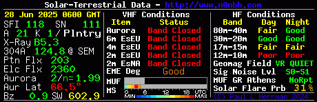 These ones.
It was then a simple matter to go back through the week, extracting the data from the images the Discord bot posted into a spreadsheet.
The challenge also asks “Did you notice any correlation between the values and the band conditions?” Well, I’ve only been on the radio a couple of times this week and the conditions weren’t great. But rather then rely on just a few subjective data points, I decided to turn the HamQSL propagation data into an estimate of “band goodness” at each point in time. On the right-hand side of the image, it lists day and night HF conditions on four groups of bands. I totaled these up, taking “poor” as 0, “fair” as 1, and “good” as 2 to produce my highly scientific “band goodness” value, which is plotted alongside the other values below.
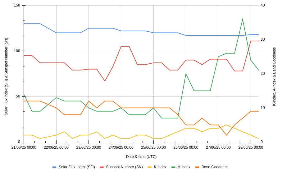 Space Weather values, 21-28 June 2025
As shown in the chart, solar flux index (SFI) and sunspot number (SN) stayed relatively constant over the week. The planetary K-index and A-index stayed low, and “Band goodness” (or propagation conditions) remained good until around Thursday, whereupon Earth passing through a “coronal hole stream” caused a spike in K-index and A-index, and a corresponding dip in HF propagation conditions.
Week 27 (30 Jun-6 Jul): Listen to the June 2025 SAQ transmission.
I will admit, I didn’t manage to cobble together a functioning receiver in time for this one. At a transmitted frequency of only 17.2 kHz, normal radio receivers aren’t suitable for the job, and it’s recommended to build a frequency converter to move the signal into an HF band. There’s also the “very amateur” suggestion to connect an antenna directly to a PC sound card, but unfortunately I discovered too late that I didn’t have a spare TRS connector to make this happen.
However, it turns out I needn’t have bothered anyway, because there was no June SAQ transmission. This year, rather than being on a Sunday as usual, the transmission has been moved to 2nd July to coincide with the site’s 100th anniversary. Unfortunately, that’s a Wednesday, so I will have to leave this challenge week for the retirees and those on holiday. I should be so lucky!
Week 28 (7-13 Jul): Receive a station on 6m via sporadic E
I do have an antenna for 6m, an HB9CV that I bought second-hand to try it portable, but then found out that it’s too heavy for my pole. Having exhausted my wife’s tolerance for antennas on the house, it sits disassembled in the shed. I had hoped to return it to service for this week’s challenge, but having been away with work all week and come down with a cold at the weekend, I had to reduce the scope of what I hoped to achieve.
My normal home HF rig is a Yaesu FT-840, a very basic model which crucially doesn’t support the 6m band. That meant I was going to have to set up another radio in order to get receiving. The FT-891 would do, but I didn’t have a suitable tuner for it to get my random wire antenna anywhere close to resonance. So, I settled for the X6100 with its capable internal tuner.
I wasn’t confident in getting out with only 10W to play with, and with my sore throat I wasn’t up for long periods of calling CQ. But the challenge was only to receive a signal via sporadic-E, so I set up for the lazy approach: radio plugged straight into the antenna, audio out from the radio to the receive half of my Signalink, and firing up WSJT-X.
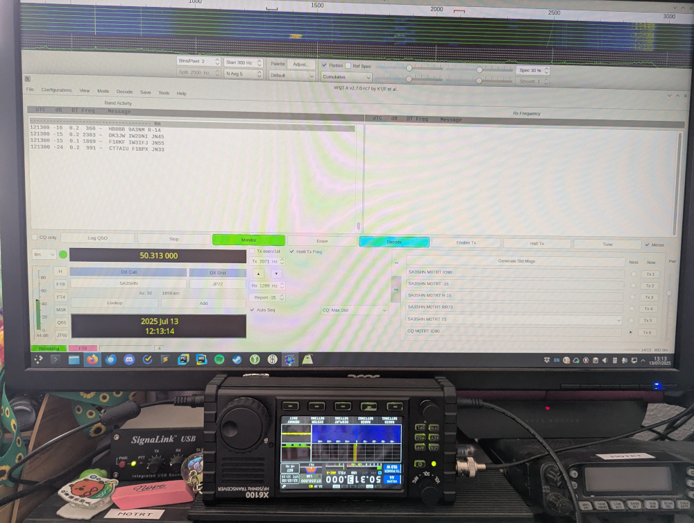
I had no way to transmit like this, but I left it running for an hour or so to see what it would pick up, then simply looked myself up on PSK Reporter to get the results.
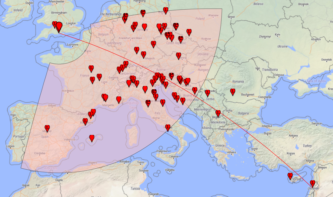
Aside from G8CEZ in Wimborne via a direct path at +22dB SNR, I heard a variety of stations across central and southern Europe via sporadic-E. Furthest DX was OD5KU in Lebanon, 3555km away and still with a perfectly serviceable -15 dB SNR. The closest station coming in via a non-direct path was F5LPL in France, at 553km, which seems a little short based on my understanding of sporadic-E; these closer-in stations may have been received via another propagation mechanism.
Surprisingly, the X6100 ATU did tune the random wire antenna to under 2:1 SWR, so perhaps in future I will give 6m sporadic-E a go with transmit capability as well through my existing antenna. That will require a bit more hardware though (or a whole new home rig to replace the aging FT-840) so onto the pile it goes for next year.
That’s all for this round-up, see you in mid-August for the results of weeks 29 to 32!
Comments